Geometry

The geometry module of gerrytools is designed to make working with different types of geometries easier. More specifcially, it is designed to to make combining subdivided geometries and generating a dual graph (which are key components to the GerryChain workflow) easier.

For this tutorial, please click on the following download link to download the necessary files:

NC Shapefile

Dual Graphs

This method allow us to generate a graph dual to the provided geometric data (a GeoDataFrame)

vtd_shp = gpd.read_file("data/NC_vtd20/") # North Carolina VTDs
graph = dualgraph(vtd_shp)

Dissolve

This dissolves the geometric data on the column by. We generally use this to dissolve a set of source geometries (e.g. VTDs, blocks, etc.) to district geometries. In this case, we’ll dissolve our North Carolina VTDs by county, since we don’t have a district assignment column.

counties = dissolve(
    geometries=vtd_shp,
    by="COUNTYFP20",
    reset_index=True, # defaults to making the result integer-indexed, not the `by` column
    keep=["TOTPOP20"], # Additional columns to keep beyond the geometry and `by` columns. Defaults to []
    aggfunc="sum", # pandas groupby function type when aggregating; defaults to "sum"
)

For a quick explanation of the parameter, we have:

• geometries: Set of geometries to be dissolved.

• by Name of the column used to group objects. In this case, we’re dissolving by county.

• reset_index If true, the index of the resulting GeoDataFrame will be set to an integer index as opposed to being indexed by the item in the by, not by. Defaults to True.

• keep A list of additional columns that we would like to keep beyond the geometry and by columns.

• aggfunc Is the aggregation function that Pandas groupby will try to call. Note: the same function is applied to all columns regardless of type.

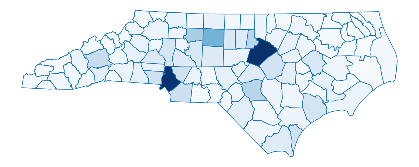
We can then easily plot the result:

fig, ax = plt.subplots(figsize=(18,8))
ax = counties.plot(
    ax=ax,
    column="TOTPOP20",
    cmap='Blues',
)
ax = counties.boundary.plot(ax=ax)
_ = plt.axis('off')

Which will produce:

Of course, remembering all of the proper syntax to make a nice matplotlib plot can be a bit tricky, so we have also made a method called chloropleth() for producing a similar plot:

from gerrytools.plotting import choropleth

counties["SHARE_OF_MAX"] = (
    counties["TOTPOP20"] / counties["TOTPOP20"].max()
)

ax = choropleth(
    geometries=counties,
    districts=counties,
    demographic_share_col="SHARE_OF_MAX",
    cmap="Blues",
    district_linecolor="#1F77B4",
    colorbar=False,
    figsize=(18,8),
)

And this code will produce:

unitmap and invert

unitmap creates a mapping from source (smaller) units to target (larger) units. invert inverts the provided unitmapping, mapping the target (larger) units to lists of source (smaller) units. Often we would want to do this for blocks → VTDs, but here we’ll test this on VTDs → counties.

mapping = unitmap((vtd_shp, "GEOID20"), (counties, "COUNTYFP20"))
inverted_mapping = invert(mapping)

print(f"mapping['37025008-00']={mapping['37025008-00']}")
print(f"inverted_mapping[25.0]={inverted_mapping[25.0]}")

Which will output:

mapping['37025008-00']=25.0
inverted_mapping[25.0]=['37025008-00', '37025001-10', '37025001-07', '37025001-08',
'37025002-08', '37025002-09', '37025003-00', '37025012-04', '37025012-03',
'37025002-06', '37025002-07', '37025002-02', '37025011-01', '37025009-00',
'37025004-01', '37025012-11', '37025004-08', '37025012-12', '37025012-08',
'37025012-09', '37025002-03', '37025001-02', '37025001-04', '37025010-00',
'37025004-03', '37025005-00', '37025012-05', '37025011-02', '37025002-05',
'37025006-00', '37025012-10', '37025002-01', '37025004-09', '37025007-00',
'37025012-06', '37025012-13', '37025004-12', '37025004-11', '37025004-13',
'37025001-11']