Plotting

The plotting module of gerrychain is designed to provide several convenience functions for visualizing the results of from a generated ensemble, and to help us to visualize the findings in terms of the geometry of the state in question.

For this tutorial, we will be working with the following shapefile of the state of Georgia:

GA Shapefile

You will also need a copy of the county file:

GA County File

Geographic Plotting

First, we will need to import all of the necessary modules and load our shapefile:

from gerrytools.scoring import *
from gerrytools.plotting import *
import pandas as pd
import geopandas as gpd
from gerrychain import Graph
import matplotlib.pyplot as plt



plan = gpd.read_file("data/GA_CD_example")

Within this module, there are functions that allow us to visualize a districting plan, as well as draw a choropleth for a certain demographic within the plan, or a dot density map of the plan.

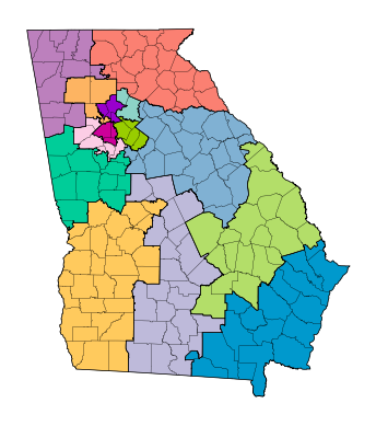
First we’ll start with drawplan. In order to use this, you will need your desired plan as a shapefile on any units with a dedicated column for districts. This function also allows us to overlay other geographies on the plan. In this case, we’re plotting a plan for the GA Congressional map, and we’ll overlay the plan with Georgia counties.

This function automatically plots the plan using districtr colors, a list of 33 colors, so if the plan has more than 33 districts, there will be repeats. A user defined color list can be passed using the colors argument, which is for the name of a column that defines color on the shapefile.

ga_county = gpd.read_file("ga_county.zip")
ga_county.columns

And we can see that the columns are:

Index(['NBAPAVAP20', 'FUNCSTAT20', 'STATEFP20', 'BVAP20', 'LOGRECNO', 'AMINVAP20',
    'COUNTYFP20', 'WPOP20', 'STUSAB', 'DOJBVAP20', 'APAMIVAP20', 'COPOP20', 'APAMIPOP20',
    'HVAP20', 'HISP20', 'ASIANPOP20', 'NAMELSAD20', 'NHPIPOP20', 'APBPOP20', 'NAME20',
    'AWATER20', 'ASIANVAP20', 'WVAP20', 'MTFCC20', 'OTHERVAP20', 'CHARITER', '2MOREVAP20',
    'APAPOP20', 'GEOID20', 'SUMLEV', 'CIFSN', '2MOREPOP20', 'CLASSFP20', 'APAVAP20',
    'AMINPOP20', 'INTPTLAT20', 'NWBHPOP20', 'NWBHVAP20', 'TOTPOP20', 'VAP20', 'CSAFP20',
    'GEOCODE', 'COUNTYNS20', 'LSAD20', 'FILEID', 'BPOP20', 'OTHERPOP20', 'NHPIVAP20',
    'ALAND20', 'APBVAP20', 'CBSAFP20', 'INTPTLON20', 'METDIVFP20', 'NBAPAPOP20',
    'COVAP20', 'geometry'], dtype='object')

We will now make a new plan from the original plan that merges all of the congressional districts of the original plan:

new_plan = plan.dissolve(by='CD').reset_index()
new_plan["CD"]

And this will output:

0     01
1     02
2     03
3     04
4     05
5     06
6     07
7     08
8     09
9     10
10    11
11    12
12    13
13    14
Name: CD, dtype: object

We can now use the nice coloring option provided to us by gerrytools to help us plot the plan:

import matplotlib.pyplot as plt
import gerrytools.plotting.colors as colors
import numpy as np

N = len(new_plan)

dists = new_plan.to_crs("EPSG:3857")
dists["CD"] = dists["CD"].astype(int)
dists=dists.sort_values(by="CD")
dists["colorindex"] = list(range(N))
dists["color"] = colors.districtr(N)

ax = drawplan(plan, assignment="CD",overlays=[ga_county])

And this will give us the following image:

If you would like to see the colors and their indices, you can print out the following view of the dataframe:

dists[["color", "CD", "colorindex"]]

Which will return:

	color	CD	colorindex
0	#0099cd	1	0
1	#ffca5d	2	1
2	#00cd99	3	2
3	#99cd00	4	3
4	#cd0099	5	4
5	#9900cd	6	5
6	#8dd3c7	7	6
7	#bebada	8	7
8	#fb8072	9	8
9	#80b1d3	10	9
10	#fdb462	11	10
11	#b3de69	12	11
12	#fccde5	13	12
13	#bc80bd	14	13

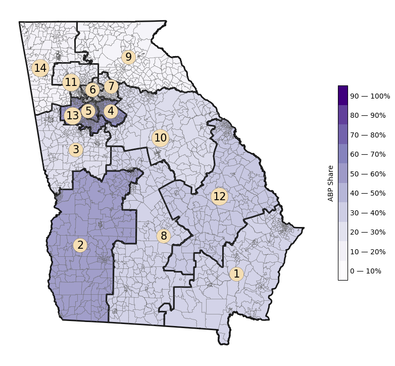
We can also draw a choropleth of a certain demographic across the map. Our drawchoropleth function takes care of this, so long as you pass a demographic share column.

You can also pass the column of total counts of any demographic share. This function plots the map, as well as a colorbar, whose label can be changed the the cbartitle argument.

plan["VAP_CD"] = plan.groupby("CD")["VAP"].transform("sum")
plan["TOTPOP_CD"] = plan.groupby("CD")["TOTPOP"].transform("sum")
plan["BVAP_SHARE_CD"] = plan["BVAP"]/plan["VAP_CD"]

districts = plan.dissolve(by="CD").reset_index()
districts["CD"] = districts["CD"].astype(int)

choro = choropleth(
    plan,
    districts=districts,
    assignment="CD",
    demographic_share_col="APB_SHARE_CD",
    overlays=[plan],
    cmap="Purples",
    cbartitle="ABP Share",
    district_lw=0.1,
    base_lw=2,
    base_linecolor="black",
    numbers=True,
)

Which gives us the following image:

Statistical Plots

Ensemble Example

We can also plot scores across an ensemble of plans. And there’s a variety of plots we’ve built in, this includes histogram(), boxplot(), and violin() plots.

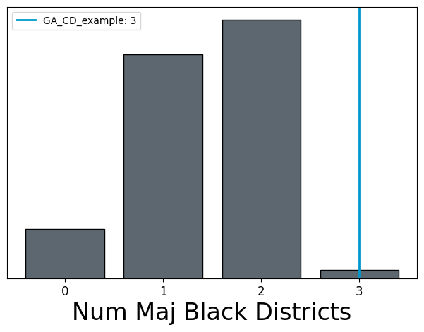
We’ll start with the histogram() function. This works by taking a dictionary with a list of scores from an ensemble, a list of scores from “citizen” maps, and a list of scores from “proposed” maps. The citizen maps will get plotted as a histogram on the same axis as the ensemble scores, while the proposed maps will appear as vertical bars with one score per plan.

In this example, we’ll plot the number of majority Black districts in an ensemble, along with one proposed map.

When using proposed maps, the argument proposed_info also has to be used. Passed to this argument is a dictionary with the keys names and colors, these will be 2 lists with the names of the proposed plans, and the desired color for their vertical line, respectively.

Let’s begin by loading in some samlpe data from a GerryChain ensemble:

import json

with open("data/ensemble_example.json") as f:
    scores = json.load(f)

scores

And this should give us:

[{'step': 1,
'BVAP20': [0.796561916484547,
0.3328762902480357,
0.04510853849452073,
0.3390029578096157,
0.08184348252955288,
0.36853268012904766,
0.3758563067575734,
0.34092315476074647,
0.16481106078363056,
0.3689490286314466,
0.27755704812900817,
0.2889411490321076,
0.14496174336179848,
0.12024937319496017],
'WVAP20': [0.6021837929440764,
0.5730542030111124,
0.6271690118945814,
0.5901055297924443,
0.6871278230021222,
0.8372431122677915,
0.5234837945593848,
0.3992002179454747,
0.6271541464343521,
0.11766183526338266,
...
0.6913443459575611,
0.6119054923551458,
0.44454273505045017,
0.698083659265221,
0.3264222628481668]}]

We now need to find the number of majority Black districts in each plan.

score_dict = {
    "ensemble": [],
    "citizen": [],
    "proposed": [],
}

for score in scores:
    count_majority_black = 0
    for apb in score["BVAP20"]:
        if apb > 0.5:
            count_majority_black += 1

    score_dict["ensemble"].append(count_majority_black)

score_dict

This code outputs:

{'ensemble': [1,
1,
2,
2,
2,
2,
2,
2,
2,
2,
2,
2,
2,
2,
2,
2,
2,
2,
2,
2,
2,
2,
2,
1,
1,
...
2,
2,
2],
'citizen': [],
'proposed': []}

We may now condense condense our starting plan down and so that we may plot the starting value on the histogram:

condensed_plan = plan[[
    "CD",
    "BVAP",
    "WVAP",
    "VAP",
    plan.geometry.name
]].dissolve(
    by="CD",
    aggfunc="sum"
)

condensed_plan["BVAP_CD"] = condensed_plan["BVAP"]/condensed_plan["VAP"]
condensed_plan["WVAP_CD"] = condensed_plan["WVAP"]/condensed_plan["VAP"]

condensed_plan

CD	geometry	BVAP	WVAP	VAP	BVAP_CD	WVAP_CD
01	POLYGON ((-82.03673…	144600	329180	516172	0.280139	0.637733
02	POLYGON ((-84.86380…	251197	233373	517382	0.485516	0.451065
03	POLYGON ((-85.08504…	111311	362833	511272	0.217714	0.709667
04	POLYGON ((-84.24440…	275786	156106	504394	0.546767	0.309492
05	POLYGON ((-84.47244…	298162	170291	536664	0.555584	0.317314
06	MULTIPOLYGON (((-84…	63904	339254	523433	0.122086	0.648133
07	POLYGON ((-84.16045…	81104	258017	486964	0.166550	0.529848
08	POLYGON ((-84.08275…	145558	337247	521602	0.279060	0.646560
09	POLYGON ((-84.25846…	32845	431576	522381	0.062876	0.826171
10	POLYGON ((-83.95610…	122589	357555	517269	0.236993	0.691236
11	MULTIPOLYGON (((-84…	72579	363918	506050	0.143423	0.719134
12	POLYGON ((-83.12176…	169050	311698	520144	0.325006	0.599253
13	MULTIPOLYGON (((-84…	264345	174182	503410	0.525109	0.346004
14	POLYGON ((-85.34267…	39916	417284	508964	0.078426	0.819869

We can now add this information into the score_dict dictionary:

score_dict["proposed"].append(
    len(condensed_plan[
        condensed_plan.BVAP_CD > 0.5
    ])
)

And plot it:

fig, ax = plt.subplots(1, 1, figsize = (7.5, 5))
hist = histogram(
    ax,
    score_dict,
    label = "Num Maj Black Districts",
    proposed_info={"names": ["GA_CD_example"]}
)

Next we’ll look at the boxplot() function. Similarly to the histogram() the scores are passed as a dictionary. However, ensemble scores must already be a lits of lists where each individual list represents the values for that box. This means that prior to plotting, scores must already be sorted and grouped so that scores are plotted lowest to highest.

Proposed plans wlll also be a list of lists. Each proposed plan list will be of length one with one score per box. An example of pre-processing to get scores in both of these formats can be seen below.

boxplot_score_dict = {"ensemble": [], "proposed": [], "citizen": []}
first_time = True
for score in scores:
    if first_time:
        for s in sorted(score["BVAP20"]):
            boxplot_score_dict["ensemble"].append([s])
        first_time = False
    else:
        for i, s in enumerate(sorted(score["BVAP20"])):
            boxplot_score_dict["ensemble"][i].append(s)
boxplot_score_dict["proposed"] = ([[k] for k in sorted(condensed_plan.APB_share)])

fig, box_ax = plt.subplots(1, 1, figsize = (7.5, 5))
box_plot = boxplot(
    box_ax,
    boxplot_score_dict,
    proposed_info={
        "names": ["GA_CD_example"],
        "colors": ["olivedrab"]
    }
)

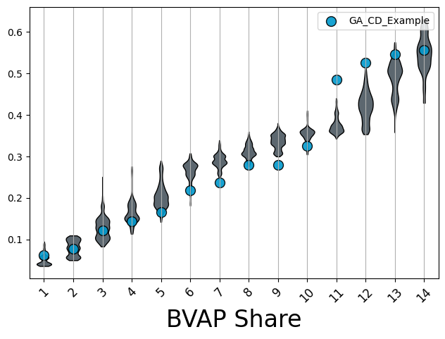
Another type of plot, similar to the boxplot, is a violin plot. These show the same information as boxplots, however, rather than data being displayed in boxes, rotated kernel densities are shown, and in some instances look like violins!

The violin() function allows us to make this plot. These takes the same score format as boxplots. In these example, we also show the use of other parameters like rotation which is a float that specifies the rotation of x axis labels. Next, we can actually define a list of 2 labels (1 for x-axis, 1 for y-axis) to be displayed on the plot.

fig, violin_ax = plt.subplots(1, 1, figsize = (7.5, 5))
violin_plot = violin(
    violin_ax,
    boxplot_score_dict,
    rotation=45,
    labels=[
        "BVAP Share",
        ""
    ],
    proposed_info={"names":["GA_CD_Example"],
    "colors":["olivedrab"]}

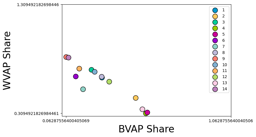
Moving away from visualizing ensembles, we can visualize specific scores about individual plans. Both the sealevel and scatter functions can be used to accomplish this. We’ll start with scatter1.

This function can be used to compare 2 scores across a plan, an ensemble, etc.

Here, we’ll compare the APBVAP20_share in each district of our example plan, and the WVAP20_share in each district of our example plan.

fig, scatter_ax = plt.subplots(1, 1, figsize = (7.5, 5))
scatter_plot = scatterplot(
    scatter_ax,
    x=[list(condensed_plan["BVAP_CD"])],
    y=[list(condensed_plan["WVAP_CD"])],
    labels = ["BVAP Share", "WVAP Share"]
)

scatter_plot.figure